Partial response curve of the pairwise most suitable community-level strategy and of the pairwise envelop of possible community-level strategy
Source:R/ellipse_plot.R
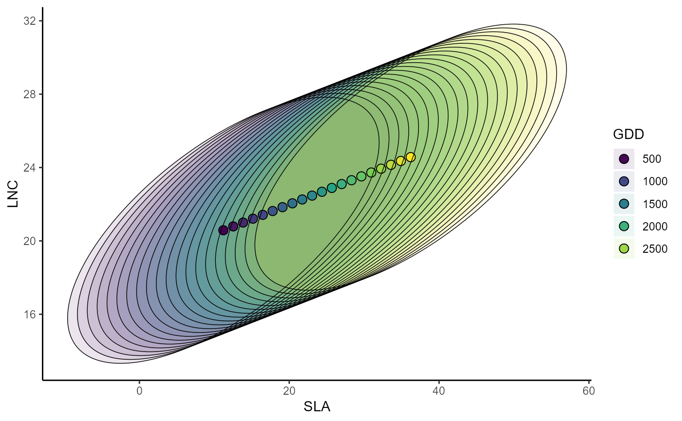
ellipse_plot.RdPartial response curve of the pairwise most suitable community-level strategy and of the pairwise envelop of possible community-level strategy. In order to build the response curve, the function builds a dataframe where the focal variable varies along a gradient and the other (non-focal) variables are fixed to their mean (but see FixX parameter for fixing non-focal variables to user-defined values). The chosen traits are specified in indexTrait. Then uses the jtdm_predict function to compute the most suitable community-level strategy and the residual covariance matrix to build the envelop of possible CWM combinations.
ellipse_plot(
  m,
  indexGradient,
  indexTrait,
  FullPost = FALSE,
  grid.length = 20,
  FixX = NULL,
  confL = 0.95
)
Arguments
- m
a model fitted with
jtdm_fit- indexGradient
The name (as specified in the column names of X) of the focal variable.
- indexTrait
A vector of the two names (as specified in the column names of Y) containing the two (or more!) traits we want to compute the community level strategy of.
- FullPost
If FullPost = TRUE, the function returns samples from the predictive distribution of joint probabilities. If FullPost= FALSE, joint probabilities are computed only using the posterior mean of the parameters.
- grid.length
The number of points along the gradient of the focal variable. Default to 20 (which ensures a fair visualization).
- FixX
Optional. A parameter to specify the value to which non-focal variables are fixed. This can be useful for example if we have some categorical variables (e.g. forest vs meadows) and we want to obtain the partial response curve for a given value of the variable. It has to be a list of the length and names of the columns of X. For example, if the columns of X are "MAT","MAP","Habitat" and we want to fix "Habitat" to 1, then FixX=list(MAT=NULL,MAP=NULL,Habitat=1.). Default to NULL.
- confL
The confidence level of the confidence ellipse (i.e. of the envelop of possible community-level strategies). Default is 0.95.
Value
Plot of the partial response curve of the pairwise most suitable community-level strategy and of the pairwise envelop of possible community-level strategy
Examples
data(Y)
data(X)
# Short MCMC to obtain a fast example: results are unreliable !
m = jtdm_fit(Y=Y, X=X, formula=as.formula("~GDD+FDD+forest"),  sample = 1000)

# plot the pairwise SLA-LNC partial response curve along the GDD gradient
ellipse_plot(m,indexTrait = c("SLA","LNC"),indexGradient="GDD")

#  plot the pairwise SLA-LNC partial response curve along the GDD gradient
#  in forest (i.e. when forest=1)
ellipse_plot(m,indexTrait = c("SLA","LNC"),indexGradient="GDD",
             FixX=list(GDD=NULL,FDD=NULL,forest=1))
# plot the pairwise SLA-LNC partial response curve along the GDD gradient
# in forest (i.e. when forest=1)
ellipse_plot(m,indexTrait = c("SLA","LNC"),indexGradient="GDD",
FixX=list(GDD=NULL,FDD=NULL,forest=1))
